본 post는 국가생명연구자원정보센터(KOBIC) 주관 서울대학교 의과대학 최무림 교수님의 WES 기초편 강의를 정리한 내용입니다.
Intro
SV(Structural Variant)의 형태와 의미를 이해합니다. SV 탐색을 위한 소프트웨어들을 알아봅니다.
De novo SV
 De novo SV
www.edwith.org/wes-beginner
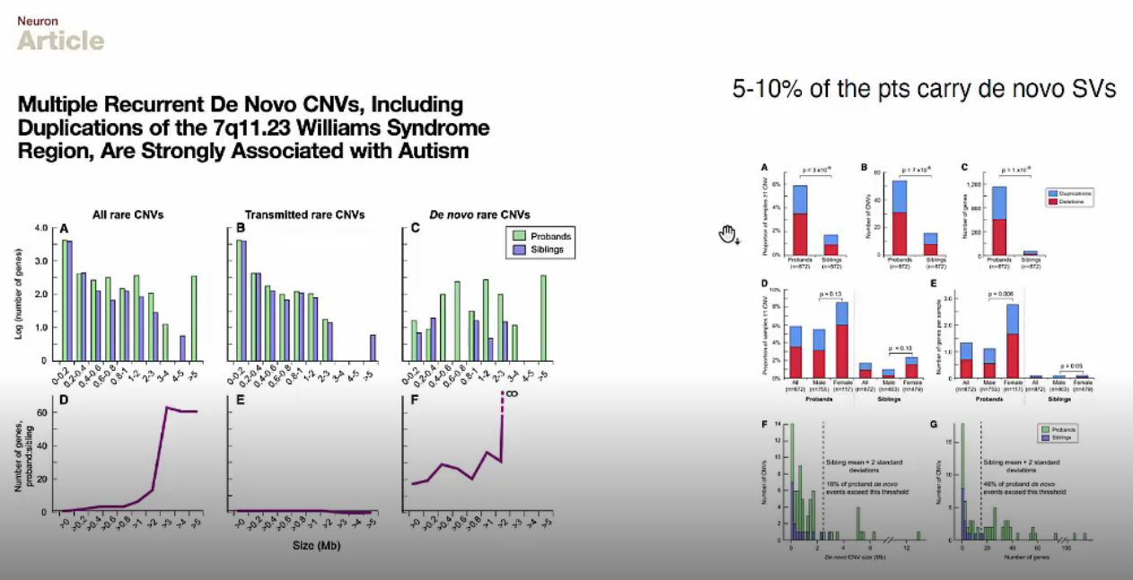
왼쪽 그래프에서 probands는 patient, siblings는 control입니다. C, F 그래프를 보면 De novo rare CNV로 인해 probands도 증가함을 확인할 수 있습니다.
오른쪽 그래프에서도 마찬가지로 5~10%의 환자가 de novo SV를 가지고 있음을 확인 했습니다.
 Calling SVs Algorithms of gnomAD
www.edwith.org/wes-beginner
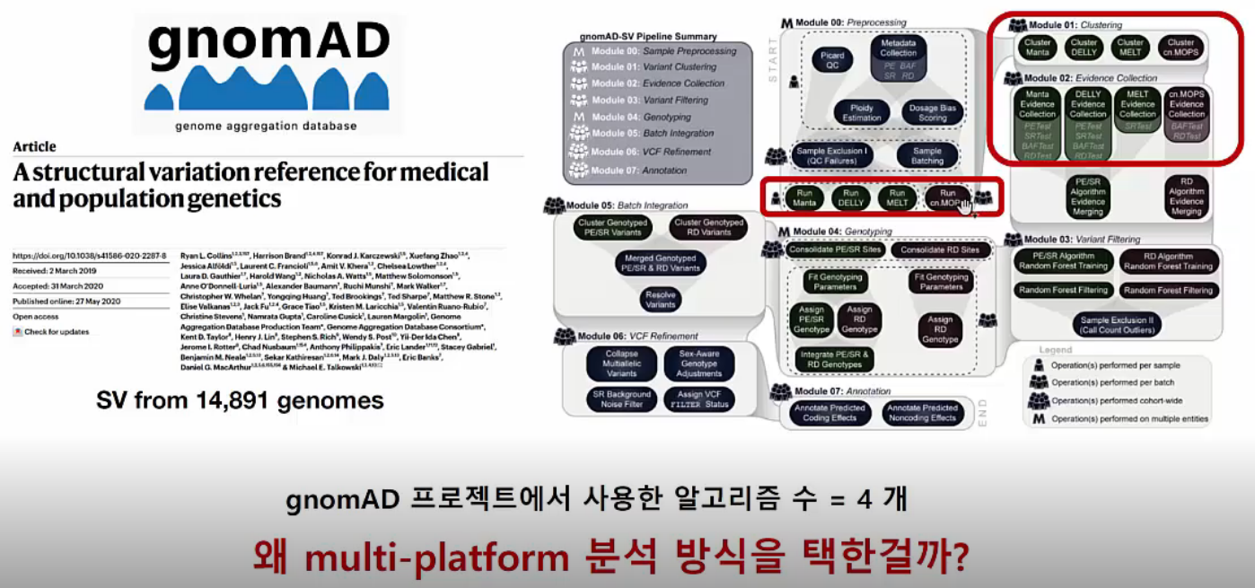
De novo SVs calling 소프트웨어는 굉장히 다양합니다. MAF Database인 gnomAD도 네 가지 algorithm으로 SV를 분석한 뒤 교집합인 SV를 사용하고 있습니다. 왜 네 가지 algorithm을 사용했는지 이어서 확인해 보겠습니다.
SV Calling Algorithms
 SV Calling Algorithms for Deletion
www.edwith.org/wes-beginner
Deletion SV calling algorithms는 다음과 같이 여러 종류가 존재합니다.
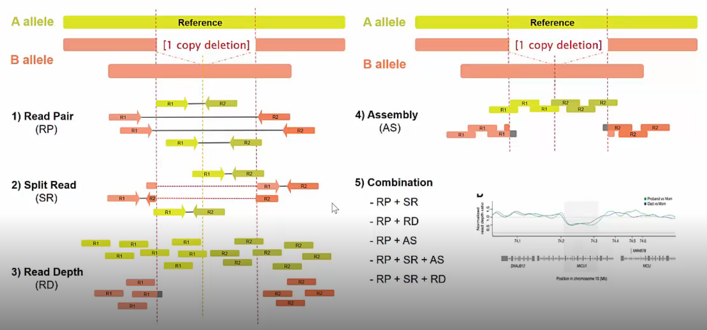
RP (Read Pair)
Paired-end sequencing 결과로 나온 r1, r2 read 사이의 insert size로 추정합니다. 예상되는 insert size (150bp~300bp)보다 훨씬 더 긴 길이를 보인다면 deletion이 존재함을 추정할 수 있습니다.
SR (Split Read)
Read 하나가 split되어 mapping 된다면 역시 deletion이 존재함을 추정할 수 있습니다.
RD (Read Depth)
Deletion이 발생한 region은 주변에 비해 read depth가 낮습니다.
AS (Assembly)
Short read들을 모아서 assembly하여 deletion이 일어난 retion을 추정할 수 있습니다.
Combination
RP+SR, RP+RD, RP+AS, RP+SR+AS, RP+SR+RD 등 다양한 조합의 algorithms로 SV를 찾아낼 수 있습니다.
 SV Calling Algorithms for Insertion
www.edwith.org/wes-beginner
Insertion SV calling algorithms는 다음과 같이 여러 종류가 존재합니다.
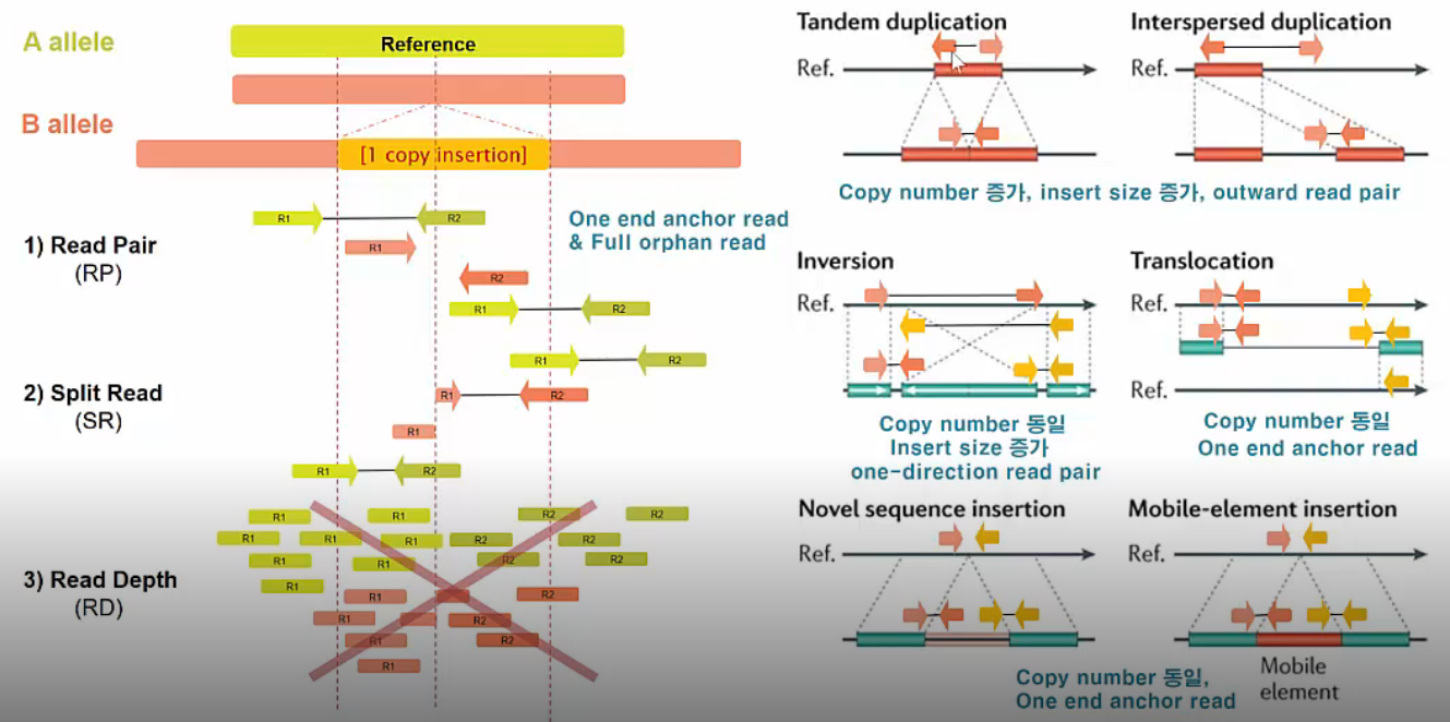
RP (Read Pair)
Paired-end sequencing 결과로 나온 r1, r2 read가 mapping되는 양상으로 insertion을 추정합니다. Paired-end read 중 하나는 reference에 mapping되고(one end anchor read) 나머지 read는 insert region에 mapping 됩니다.(full orphan read)
SR (Split Read)
One end anchor read가 split되어 mapping 된다면 역시 insertion이 존재함을 추정할 수 있습니다.
RD (Read Depth)
Insertion은 RD로 확인할 수 없습니다. Insert region을 읽은 read는 mapping 될 수 없고 일부 걸친 read만 mapping 가능하기 때문입니다. 즉, RD의 차이가 거의 없습니다.
이 외에도 Tandem duplication, Interspersed duplication, Inversion, Translocation, Novel sequence insertion, Mobile-element insertion 등의 SVs가 존재합니다.
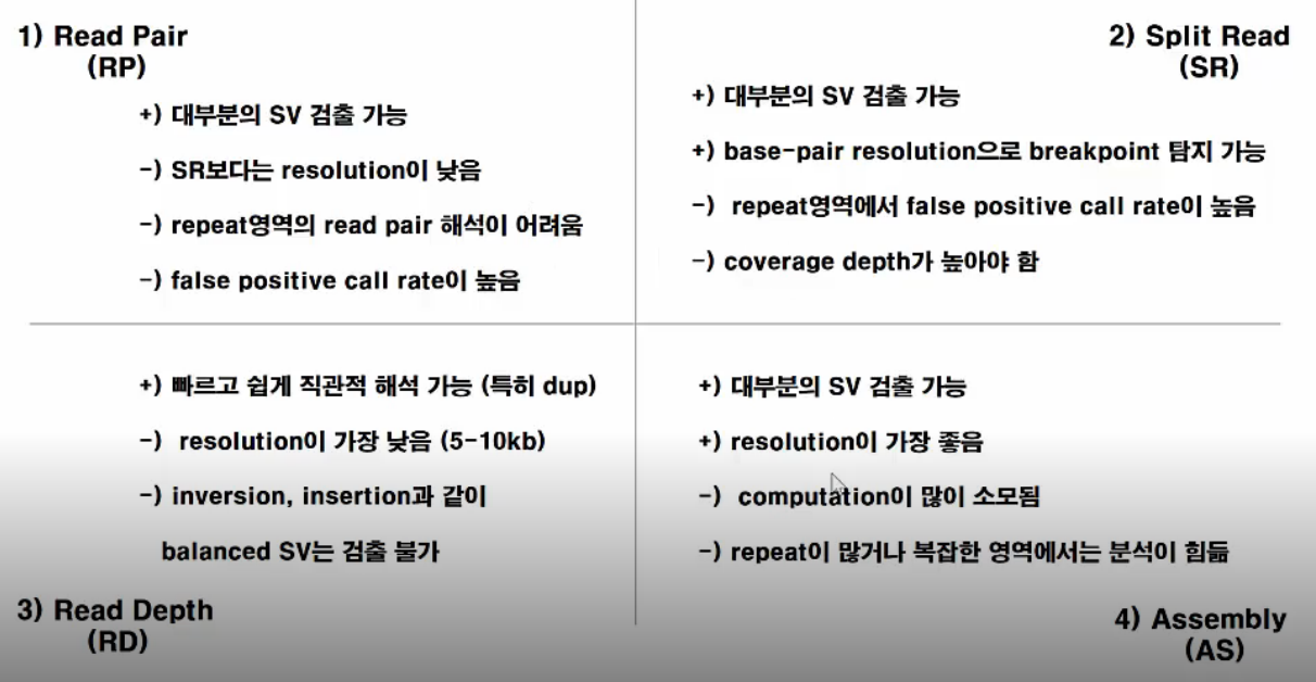
SVs callling algorithms 유형별 장단점은 아래와 같습니다. RD가 직관적이며 빠르고 쉽게 해석 가능하지만 resolution이 가장 낮습니다. RP, SR, AS로 갈수록 resolution은 늘어나지만 conputation resource가 많이 소모됩니다. 또한 공통적으로 repeat region에서의 SV calling은 어렵고 false positive ratio가 증가하므로, 소프트웨어에서 나온 SV result를 IGV 등을 통해 직접 repeat region 여부와 FP 가능성 확인이 필요합니다.
 SV Calling Algorithms: Pros & Cons
www.edwith.org/wes-beginner
Algorithms 유형별 소프트웨어 종류는 다음과 같습니다. Bold체 네 개 소프트웨어는 gnomAD에서 사용한 네 가지 소프트웨어입니다.
- RP(Read Pair): 1-2-3-SV, BreakDancer, Ulysses
- SR(Split Read): Pindel, SVseq2, Sprites
- RD(Read Depth): BICseq2, CNVantor, PennCNV-seq, cn.MPOS, readDepth
- AS(Assembly): laSV, FermiK, BreakSeek
- RP+SR: SoftSV, Wham, DELLY, Meerkat, MELT, PRISM
- RP+RD: inGAP-sv, GASVPro, forests
- RP+AS: Hydra, CREST
- RP+SR+AS: GRIDSS, Manta, SvABA
- RP+SR+RD: Lympy, MATOHCUP, TIDDIT, Svelter
소프트웨어별 SV 결과의 bias 편차가 심하기 때문에 biasgnomAD는 네 개 소프트웨어를 사용하여 편차를 줄였습니다. 이처럼 multi-platform 방식으로 보완이 가능합니다.
Manta: De novo Deletion Result
 Manta: De novo Deletion
www.edwith.org/wes-beginner
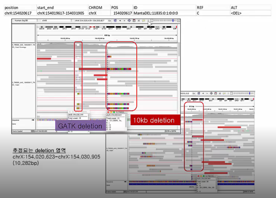
Manta 소프트웨어로 분석한 결과 중 de novo deletion을 IGV로 확인한 결과입니다. De novo deletion이 존재하는 region에서 soft-clipped reads가 확인됩니다.
 Manta: De novo Deletion
www.edwith.org/wes-beginner
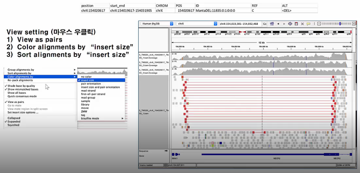
Insert size 크기로 coloring한 뒤 sorting한 결과입니다. 마찬가지로 de novo deletion이 존재하는 region에서 insert size가 큰 reads가 확인됩니다.
Summary
- SV는 비록 많은 비율은 아니지만 대부분의 disease 유발 인자로 생각되고 있습니다.
- SV calling은 SNV보다 어렵고 독립적인 algorithm을 사용해야 합니다.
- SV calling 결과에 대한 후속 확인이 필수적입니다.