Gambler’s Ruin 문제를 계차방정식을 이용해 풀고, 확률변수의 정의를 이해할 수 있습니다.
Gambler’s Ruin
A, B 두 명의 gambler가 내기를 합니다. 매 round에서 1 dollar를 걸고 내기에서 이긴 사람이 가져갑니다. A는 i dollar, B는 (N-i) dollar를 가지고 시작합니다.
p = A가 이길 확률
q = B가 이길 확률 = 1-p
Random Walk
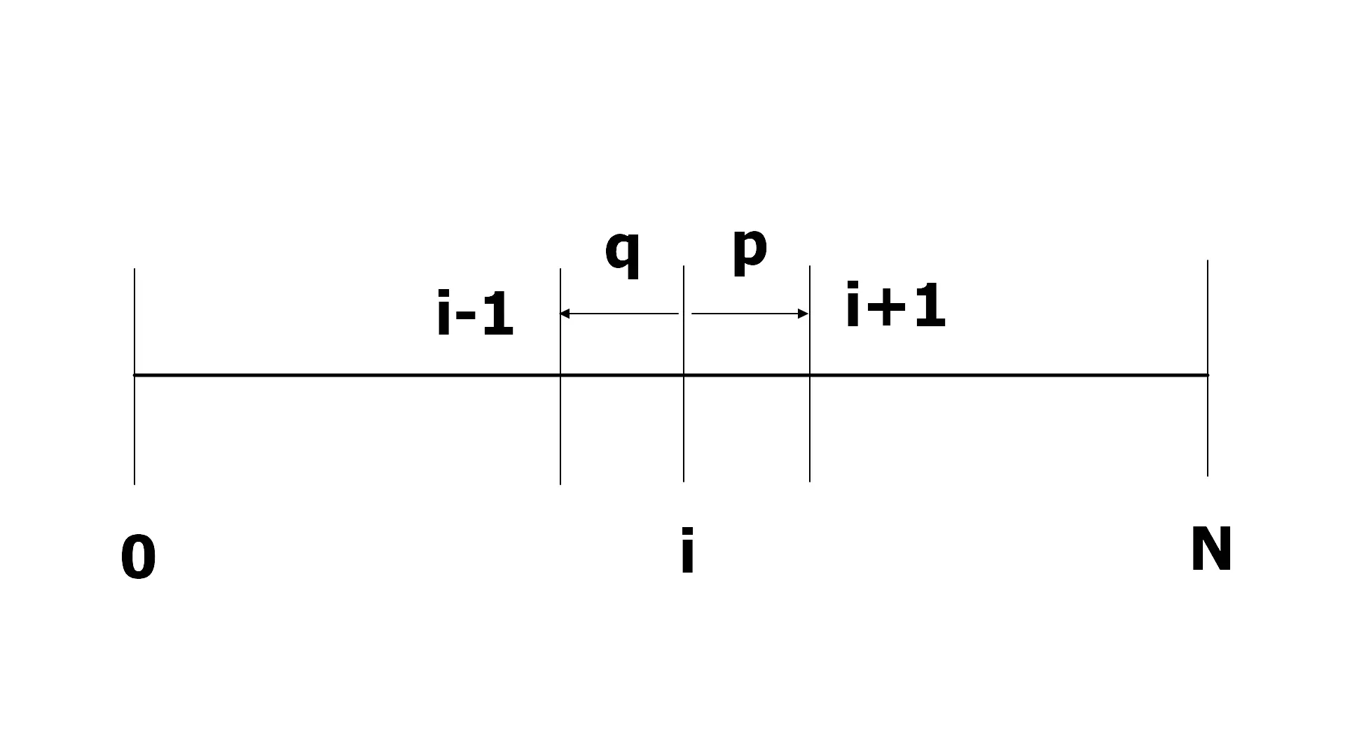
위 문제는 유형을 파악하는 것이 중요합니다. 이와 같은 유형의 문제는 random walk로 정의할 수 있습니다.
p는 오른쪽으로 이동할 확률, q는 왼쪽으로 이동할 확률입니다. 0, N은 absorbing state로 갇힌 상태입니다.
Strategy: Condition on first step
Pi=P(Awinsgame∣Astartsatidollar)
Pi=pPi+1+qPi−1, (1≤i≤N−1), (p0=0,pN=1)
문제를 해결하는데 가장 중요한 식입니다. Difference qeuation(계차방정식)이라고 부르며 미분방정식의 이산 형태입니다.
Guessing을 통한 풀이
Pi=xi
xi=pxi+1+qxi−1
px2−x+q=0
x=2p1±1−4pq∈{1,pq}
두 해가 다른 경우(p=q)
두 해의 선형결합 식으로 표현할 수 있습니다. pi=A1i+B(pq)i,(p=q)
조건 p0=0,pN=1을 대입하면, p0=A+B=0, B=−A pN=A+B(pq)N=A(1−(pq)N)=1 A=1−(pq)N1 pi=1−(pq)N−11−(pq)i,(p=q)
두 해가 같은 경우(p=q) x=pq로 치환하고 x→1의 극한을 살펴봅니다. limx→11−xN1−xi=limx→1N(xN−1)i(xi−1)=Ni
카지노(A)와 gambler(B)가 같은 돈을 가지고 시작했을 때 카지노에게 1%라도 유리한 게임인 경우 gambler가 이길 확률은 매우 작아집니다.
i=N−i,p=0.49 N=20→0.40 N=100→0.12 N=200→0.02
Random Variables (확률변수)
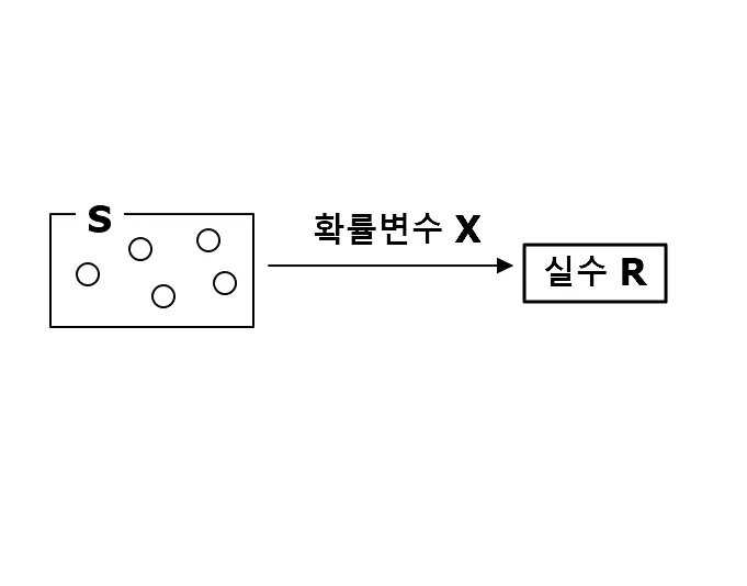
우선 확률변수의 정의를 알아봅시다. 확률변수는 function입니다. 이 function은 표본공간 S로부터 실수 체계 R로 mapping합니다.
쉽고 중요한 예제들을 살펴봅니다.
Bernoulli (베르누이) 확률분포
A random variable X is said to have Bernoulli(p) distribution, if X has only 2 possible values, 0 and 1
P(X=1) = p
P(X=0) = 1-P
Binomial (이항) 확률분포 (n,p)
The distribution of #success X in n independent Bernoulli(p) trials is called Binomial(n,p), its distribution is given by P(X=k)=(kn)pk(1−p)n−k
이 식은 PMF(확률질량변수)라고 합니다.
XBin(n,p), YBin(m,p), X와 Y가 independent일 때 X+Y~Bin(n+m, p)를 따릅니다.
IMO
Difference equation(계차방정식)을 다루는 곳이 거의 없는데 중요한 개념으로 보입니다. 베르누이분포, 이항분포를 시작으로 확률변수 분포가 나오는데 잘 정리해야 겠습니다.