Dataframe in Pandas
Intro
Pandas는 data analysis에 유용한 python package 입니다. Pandas는 쉽고 편리하게 data를 다룰 수 있도록 유연한 structure를 제공하는데, 그 중 하나가 바로 Dataframe 입니다.
이 post는 pandas 공식 가이드 내 10 minutes to pandas를 참고 했습니다.
Dataframe이란?
Dataframe은 data를 직사각형 모양 table에 저장한 구조입니다. Row는 숫자, 문자, 논리 등 여러 가지 data type이 들어갈 수 있습니다. Column은 동일한 data type이 들어갈 수 있습니다. 즉, 각 column에 아마도 서로 다른 data type을 지닌 2d array data 구조로 요약할 수 있습니다. 참고로 1d array data 구조는 Series 입니다.
R 언어를 알고 계시는 분들은 data.frame이 친숙할 것입니다. Pandas의 dataframe과 유사한 구조입니다.
Dataframe의 주요 요소입니다.
-
Data: Dataframe 자체가 들어갈 수 있고 그 외 series, numpy의 ndarray, 2d ndarray, dictionary가 들어갈 수 있습니다.
-
Index: Numpy의 array나 2d array와 비슷하지만, dataframe에는 index가 존재한다는 차이가 있습니다.
-
Column: Column의 index도 존재하여 data를 손쉽게 다룰 수 있도록 도와줍니다.
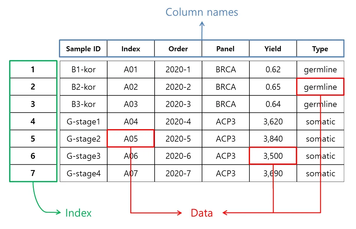 Dataframe 주요 요소
Manipulating Dataframe
Object creation
Dataframe을 생성합니다.
Import required libraries
Numpy와 Pandas를 import 합니다.
import numpy as np
import pandas as pd
Object creation
pandas에 list를 넘겨 ‘Series’를 만들어 봅시다.
Index는 기본 설정을 사용합니다. 0부터 시작하여 1씩 증가합니다.
s = pd.Series([1, 3, 5, 7, 9])
s
0 1
1 3
2 5
3 7
4 9
dtype: int64pandas에 NumPy array를 넘겨 ‘DataFrame’을 만들어 봅시다.
Index는 연속된 날짜를, column name은 A, B, C를 사용합니다.
dates = pd.date_range('20200717', periods=6)
dates
DatetimeIndex(['2020-07-17', '2020-07-18', '2020-07-19', '2020-07-20',
'2020-07-21', '2020-07-22'],
dtype='datetime64[ns]', freq='D')df = pd.DataFrame(
np.random.randn(6, 3), # NumPy array
index=dates,
columns=list('ABC')
)
df A B C
2020-07-17 -0.649036 1.194016 -1.671976
2020-07-18 -0.551816 -2.254361 -0.109569
2020-07-19 -0.914518 -0.385325 0.259745
2020-07-20 -0.029484 0.119984 -0.299513
2020-07-21 -0.302863 0.004918 -0.671543
2020-07-22 -0.615118 -1.382085 0.226391pandas에 series와 유사하게 변형될 수 있는 형태의 dictionary를 넘겨 ‘DataFrame’을 만들어 봅시다.
Index는 기본 설정이, column name은 dictionary의 key가 들어갑니다.
df2 = pd.DataFrame({
            'A': 1.,
            'B': pd.Timestamp('20200701'),
            'C': pd.Series(1, index=list(range(4)), dtype='float32'),
            'D': np.array([3] * 4, dtype='int32'),
            'E': pd.Categorical(["test", "train", "test", "train"]),
            'F': 'foo'
            })
df2
A B C D E F
0 1.0 2020-07-01 1.0 3 test foo
1 1.0 2020-07-01 1.0 3 train foo
2 1.0 2020-07-01 1.0 3 test foo
3 1.0 2020-07-01 1.0 3 train foodf2는 column별로 다른 data type으로 구성되어 있습니다.
소수점은 ‘float64’, 문자는 ‘object’ 자료형이 할당됩니다.
df2.dtypesA float64
B datetime64[ns]
C float32
D int32
E category
F object
dtype: objectdf2.<TAB> 혹은 dir(df2)를 실행하면 DataFrame(df2)이 가지고 있는 속성을 확인할 수 있습니다.
dir(df2)['A',
'B',
'C',
'...',
'var',
'where',
'xs']Viewing data
생성한 dataframe을 확인합니다. 간단한 statistics summary, 행렬변환, 정렬 등을 시도해 보겠습니다.
앞서 진행한 import와 DataFrame 생성을 반복합니다.
import numpy as np
import pandas as pd

dates = pd.date_range('20200724', periods=6)
df = pd.DataFrame(
        np.random.randn(6, 4),
        index=dates,
        columns=list('ABCD')
        )
Viewing data
DataFrame의 처음과 끝 부분을 출력해 봅시다.
df.head() A B C D
2020-07-24 -0.165906 1.178056 0.018960 0.032754
2020-07-25 -0.194626 0.387675 0.400168 0.236478
2020-07-26 -0.667234 -0.513509 -1.760879 -1.337563
2020-07-27 -1.291120 0.151518 0.231840 0.066671
2020-07-28 0.229097 1.285831 -0.852687 0.366998df.tail(3) A B C D
2020-07-27 -1.291120 0.151518 0.231840 0.066671
2020-07-28 0.229097 1.285831 -0.852687 0.366998
2020-07-29 1.640661 -0.006239 0.494051 -1.189063DataFrame의 index와 column name도 출력해 봅시다.
df.indexDatetimeIndex(['2020-07-24', '2020-07-25', '2020-07-26', '2020-07-27',
'2020-07-28', '2020-07-29'],
dtype='datetime64[ns]', freq='D')df.columnsIndex(['A', 'B', 'C', 'D'], dtype='object')describe()는 DataFrame의 요약통계치를 빠르게 보여줍니다.
df.describe() A B C D
count 6.000000 6.000000 6.000000 6.000000
mean -0.074855 0.413889 -0.244758 -0.303954
std 0.988760 0.700048 0.886190 0.754287
min -1.291120 -0.513509 -1.760879 -1.337563
25% -0.549082 0.033200 -0.634775 -0.883609
50% -0.180266 0.269597 0.125400 0.049712
75% 0.130346 0.980461 0.358086 0.194027
max 1.640661 1.285831 0.494051 0.366998DataFrame의 행과 열을 뒤바꿀 수도 있습니다.
df.T 2020-07-24 2020-07-25 2020-07-26 2020-07-27 2020-07-28 2020-07-29
A -0.165906 -0.194626 -0.667234 -1.291120 0.229097 1.640661
B 1.178056 0.387675 -0.513509 0.151518 1.285831 -0.006239
C 0.018960 0.400168 -1.760879 0.231840 -0.852687 0.494051
D 0.032754 0.236478 -1.337563 0.066671 0.366998 -1.189063DataFrame의 정렬기능은 index에 따라, column name에 따라, 혹은 특정 value에 따라 가능합니다.
df.sort_index() # sorting by index A B C D
2020-07-24 -0.165906 1.178056 0.018960 0.032754
2020-07-25 -0.194626 0.387675 0.400168 0.236478
2020-07-26 -0.667234 -0.513509 -1.760879 -1.337563
2020-07-27 -1.291120 0.151518 0.231840 0.066671
2020-07-28 0.229097 1.285831 -0.852687 0.366998
2020-07-29 1.640661 -0.006239 0.494051 -1.189063df.sort_index(axis=1, ascending=False) # sorting by column name in descending order D C B A
2020-07-24 0.032754 0.018960 1.178056 -0.165906
2020-07-25 0.236478 0.400168 0.387675 -0.194626
2020-07-26 -1.337563 -1.760879 -0.513509 -0.667234
2020-07-27 0.066671 0.231840 0.151518 -1.291120
2020-07-28 0.366998 -0.852687 1.285831 0.229097
2020-07-29 -1.189063 0.494051 -0.006239 1.640661df.sort_values(by='B') # sorting by values in 'B' column A B C D
2020-07-26 -0.667234 -0.513509 -1.760879 -1.337563
2020-07-29 1.640661 -0.006239 0.494051 -1.189063
2020-07-27 -1.291120 0.151518 0.231840 0.066671
2020-07-25 -0.194626 0.387675 0.400168 0.236478
2020-07-24 -0.165906 1.178056 0.018960 0.032754
2020-07-28 0.229097 1.285831 -0.852687 0.366998Selection
Data를 선택하고 변경하는 방법입니다.
앞서 진행한 import와 DataFrame 생성을 반복합니다.
import numpy as np
import pandas as pd

dates = pd.date_range('20200724', periods=6)
df = pd.DataFrame(
        np.random.randn(6, 4),
        index=dates,
        columns=list('ABCD')
        )
Data를 분석하려면 특정 값을 선택해서 다루거나 출력할 필요가 있습니다.
이 때 사용할 수 있는 기능들을 살펴 보겠습니다.
Getting
하나의 column을 선택합니다. ‘Series’ 형태의 결과를 생성합니다.
df['A'] # selecting a single column2020-07-24 0.769295
2020-07-25 -0.501942
2020-07-26 -1.569191
2020-07-27 -0.861305
2020-07-28 1.572154
2020-07-29 -0.287700
Freq: D, Name: A, dtype: float64[ ]를 이용하여 복수의 행을 잘라 선택할 수 있습니다.
df[0:3] # selecting rows A B C D
2020-07-24 0.769295 0.844431 -0.918174 -0.047887
2020-07-25 -0.501942 0.097646 -0.963513 -0.260229
2020-07-26 -1.569191 0.257844 -1.276382 0.620355
df['2020-07-25':'2020-07-28'] # selecting rows A B C D
2020-07-25 -0.501942 0.097646 -0.963513 -0.260229
2020-07-26 -1.569191 0.257844 -1.276382 0.620355
2020-07-27 -0.861305 -0.123141 -0.729888 0.465927
2020-07-28 1.572154 0.227942 0.125129 0.278978Selection by label
Index name이나 column name으로 선택할 수 있습니다.
‘loc’을 사용합니다.
첫 번째 Index에 해당하는 모든 데이터를 가져와 보겠습니다.
df.loc[dates[0]]A 0.769295
B 0.844431
C -0.918174
D -0.047887
Name: 2020-07-24 00:00:00, dtype: float64두 개의 column name에 해당하는 모든 데이터를 가져와 보겠습니다.
df.loc[:, ['A', 'B']] A B
2020-07-24 0.769295 0.844431
2020-07-25 -0.501942 0.097646
2020-07-26 -1.569191 0.257844
2020-07-27 -0.861305 -0.123141
2020-07-28 1.572154 0.227942
2020-07-29 -0.287700 0.835631이번에는 index name과 column name 모두 조건에 만족하는 데이터를 가져와 보겠습니다.
df.loc['2020-07-25':'2020-07-26', ['A', 'B']] A B
2020-07-25 -0.501942 0.097646
2020-07-26 -1.569191 0.257844
df.loc['2020-07-25', ['A', 'B']]A -0.501942
B 0.097646
Name: 2020-07-25 00:00:00, dtype: float64특정 위치의 한 개 값을 가져와 보겠습니다.
‘loc’과 ‘at’ 모두 사용할 수 있습니다.
df.loc[dates[0], 'A']0.7692952378187148
df.at[dates[0], 'A']0.7692952378187148Selection by position
이번에는 index와 column 모두 위치를 기준으로 데이터를 선택하는 방법에 대해서 알아보겠습니다.
여기서 사용하는 위치는 python에서 사용하는 index 개념과 동일합니다.
‘iloc’을 사용합니다.
먼저 하나의 단일 위치를 사용할 수 있습니다.
df.iloc[3]A -0.861305
B -0.123141
C -0.729888
D 0.465927
Name: 2020-07-27 00:00:00, dtype: float64다음은 행과 열 모두 범위 단위 인덱스 정보를 사용한 예 입니다.
df.iloc[3:5, 0:2] A B
2020-07-27 -0.861305 -0.123141
2020-07-28 1.572154 0.227942또한 list 형태로 위치를 사용할 수도 있습니다.
df.iloc[
        [1, 2, 4],
        [0, 2]
        ]
A C
2020-07-25 -0.501942 -0.963513
2020-07-26 -1.569191 -1.276382
2020-07-28 1.572154 0.125129label을 사용했을 때와 마찬가지로 행이나 열을 선택할 수도 있습니다.
df.iloc[1:3, :] # selecting by row index A B C D
2020-07-25 -0.501942 0.097646 -0.963513 -0.260229
2020-07-26 -1.569191 0.257844 -1.276382 0.620355
df.iloc[:, 1:3] # selecting by column index B C
2020-07-24 0.844431 -0.918174
2020-07-25 0.097646 -0.963513
2020-07-26 0.257844 -1.276382
2020-07-27 -0.123141 -0.729888
2020-07-28 0.227942 0.125129
2020-07-29 0.835631 1.684919역시 특정 위치를 선택하여 하나의 value만 선택할 수도 있습니다.
‘iloc’과 ‘iat’ 모두 사용할 수 있습니다.
df.iloc[1, 1]0.09764616018895249
df.iat[1, 1]0.09764616018895249Boolean indexing
논리에 따라 해당되는 값을 선택하는 방법을 알아보겠습니다.
특정 column의 값들 중 조건에 해당하는 data만 선택하는 방법입니다.
df[df['A'] > 0] # select if the 'A' columne's value is greater than 0 A B C D
2020-07-24 0.769295 0.844431 -0.918174 -0.047887
2020-07-28 1.572154 0.227942 0.125129 0.278978전체 DataFrame 값 중 조건을 충족하는 data만 선택할 수도 있습니다.
이 때 조건을 충족하지 못하는 data는 모두 NaN으로 표기됩니다.
df[df > 0] A B C D
2020-07-24 0.769295 0.844431 NaN NaN
2020-07-25 NaN 0.097646 NaN NaN
2020-07-26 NaN 0.257844 NaN 0.620355
2020-07-27 NaN NaN NaN 0.465927
2020-07-28 1.572154 0.227942 0.125129 0.278978
2020-07-29 NaN 0.835631 1.684919 0.506765isin() method를 사용해서 filter 할 수도 있습니다.
df2 = df.copy()
df2['E'] = ['one', 'one', 'two', 'three', 'four', 'three']
df2
A B C D E
2020-07-24 0.769295 0.844431 -0.918174 -0.047887 one
2020-07-25 -0.501942 0.097646 -0.963513 -0.260229 one
2020-07-26 -1.569191 0.257844 -1.276382 0.620355 two
2020-07-27 -0.861305 -0.123141 -0.729888 0.465927 three
2020-07-28 1.572154 0.227942 0.125129 0.278978 four
2020-07-29 -0.287700 0.835631 1.684919 0.506765 three
df2[df2['E'].isin(['two', 'four'])] # select if the 'E' column's value is 'two' or 'four' A B C D E
2020-07-26 -1.569191 0.257844 -1.276382 0.620355 two
2020-07-28 1.572154 0.227942 0.125129 0.278978 fourSetting
DataFrame의 data를 변경할 수 있습니다.
먼저 DataFrame에 새로운 column을 추가하는 방법을 알아보겠습니다.
index를 가지고 있는 Series를 만들고 DataFrame의 새로운 column을 지정하여 추가할 수 있습니다.
new_s1 = pd.Series(
        [1, 2, 3, 4, 5, 6],
        index=pd.date_range('20200725', periods=6)
        )

new_s1
2020-07-25 1
2020-07-26 2
2020-07-27 3
2020-07-28 4
2020-07-29 5
2020-07-30 6
Freq: D, dtype: int64
df['F'] = new_s1 # assign Series to DataFrame's 'F' column

df
A B C D F
2020-07-24 0.769295 0.844431 -0.918174 -0.047887 NaN
2020-07-25 -0.501942 0.097646 -0.963513 -0.260229 1.0
2020-07-26 -1.569191 0.257844 -1.276382 0.620355 2.0
2020-07-27 -0.861305 -0.123141 -0.729888 0.465927 3.0
2020-07-28 1.572154 0.227942 0.125129 0.278978 4.0
2020-07-29 -0.287700 0.835631 1.684919 0.506765 5.0label을 사용하여 data를 수정할 수도 있습니다.
df.at[dates[0], 'A'] = 0
df
A B C D F
2020-07-24 0.000000 0.844431 -0.918174 -0.047887 NaN
2020-07-25 -0.501942 0.097646 -0.963513 -0.260229 1.0
2020-07-26 -1.569191 0.257844 -1.276382 0.620355 2.0
2020-07-27 -0.861305 -0.123141 -0.729888 0.465927 3.0
2020-07-28 1.572154 0.227942 0.125129 0.278978 4.0
2020-07-29 -0.287700 0.835631 1.684919 0.506765 5.0위치 정보를 사용하여 data를 수정할 수도 있습니다.
df.iat[0, 1] = 0
df
A B C D F
2020-07-24 0.000000 0.000000 -0.918174 -0.047887 NaN
2020-07-25 -0.501942 0.097646 -0.963513 -0.260229 1.0
2020-07-26 -1.569191 0.257844 -1.276382 0.620355 2.0
2020-07-27 -0.861305 -0.123141 -0.729888 0.465927 3.0
2020-07-28 1.572154 0.227942 0.125129 0.278978 4.0
2020-07-29 -0.287700 0.835631 1.684919 0.506765 5.0data를 수정할 때 numpy array를 대응시켜 특정 column data를 모두 수정할 수도 있습니다.
df.loc[:, 'D'] = np.array([5] * len(df))
df
A B C D F
2020-07-24 0.000000 0.000000 -0.918174 5 NaN
2020-07-25 -0.501942 0.097646 -0.963513 5 1.0
2020-07-26 -1.569191 0.257844 -1.276382 5 2.0
2020-07-27 -0.861305 -0.123141 -0.729888 5 3.0
2020-07-28 1.572154 0.227942 0.125129 5 4.0
2020-07-29 -0.287700 0.835631 1.684919 5 5.0마지막으로 조건에 해당하는 data 값들을 모두 음수로 변환해 보겠습니다.
df2 = df.copy()
df2[df2 > 0] = -df2
df2
A B C D F
2020-07-24 0.000000 0.000000 -0.918174 -5 NaN
2020-07-25 -0.501942 -0.097646 -0.963513 -5 -1.0
2020-07-26 -1.569191 -0.257844 -1.276382 -5 -2.0
2020-07-27 -0.861305 -0.123141 -0.729888 -5 -3.0
2020-07-28 -1.572154 -0.227942 -0.125129 -5 -4.0
2020-07-29 -0.287700 -0.835631 -1.684919 -5 -5.0Missing data
결측치를 확인하고 처리하는 방법입니다.
앞서 진행한 import와 DataFrame 생성을 반복합니다.
import numpy as np
import pandas as pd

dates = pd.date_range('20200724', periods=6)
df = pd.DataFrame(
        np.random.randn(6, 4),
        index=dates,
        columns=list('ABCD')
        )
pandas에서는 결측치(missing data)를 주로 ‘np.nan’으로 표현합니다.
이번에는 결측치(missing data)를 다루는 방법에 대해 살펴보겠습니다.
‘reindex’는 특정 column의 index를 수정/추가/삭제 할 수 있습니다.
그 결과 복사된 DataFrame을 반환합니다.
df1 = df.reindex(
        index=dates[0:4],
        columns=list(df.columns) + ['E']
        )
df1.loc[dates[0]:dates[1], 'E'] = 1
df1
A B C D E
2020-07-24 0.301247 -0.425514 -1.233032 0.259611 1.0
2020-07-25 1.090123 -1.035311 1.168112 -1.214599 1.0
2020-07-26 1.266217 0.809175 -0.578900 -0.658111 NaN
2020-07-27 -0.911602 0.208199 0.596766 1.066030 NaNmissing data가 하나라도 포함된 행을 제외시켜 봅시다.
‘dropna’를 사용합니다.
df1.dropna(how='any') A B C D E
2020-07-24 0.301247 -0.425514 -1.233032 0.259611 1.0
2020-07-25 1.090123 -1.035311 1.168112 -1.214599 1.0missing data를 특정 값으로 채워봅시다.
‘fillna’를 사용합니다.
df1.fillna(value=5) A B C D E
2020-07-24 0.301247 -0.425514 -1.233032 0.259611 1.0
2020-07-25 1.090123 -1.035311 1.168112 -1.214599 1.0
2020-07-26 1.266217 0.809175 -0.578900 -0.658111 5.0
2020-07-27 -0.911602 0.208199 0.596766 1.066030 5.0data 값이 ‘nan’인지 아닌지 확인만 해봅시다.
‘isna’를 사용합니다.
pd.isna(df1) A B C D E
2020-07-24 False False False False False
2020-07-25 False False False False False
2020-07-26 False False False False True
2020-07-27 False False False False TrueOperations
본격적으로 data를 다뤄봅니다. Statistics를 구하고 사칙연산 function을 적용합니다.
앞서 진행한 import와 DataFrame 생성을 반복합니다.
import numpy as np
import pandas as pd

dates = pd.date_range('20200724', periods=6)
df = pd.DataFrame(
        np.random.randn(6, 4),
        index=dates,
        columns=list('ABCD')
        )
df
A B C D
2020-07-24 -0.910768 0.416166 0.197304 0.252876
2020-07-25 0.615104 1.164349 0.044059 -1.996138
2020-07-26 -1.354868 -0.017010 -0.784717 1.337247
2020-07-27 -0.414421 0.992017 1.257737 -0.361511
2020-07-28 -0.194671 -1.427558 0.896521 0.110179
2020-07-29 1.486213 0.975022 -0.125846 1.531045DataFrame의 연산을 살펴보겠습니다.
Stats
일반적으로 연산에서 missing data는 제외합니다.
우선 기술통계(descriptive statistic)를 수행해 보겠습니다.
각 column 별로 평균값을 구해봅시다.
df.mean()A 0.231753
B -0.123741
C 0.078004
D -0.031127
dtype: float64이번에는 각 index 별로 평균값을 구해봅시다.
df.mean(1)2020-07-24 0.410100
2020-07-25 -0.124489
2020-07-26 0.140944
2020-07-27 -0.362837
2020-07-28 0.360954
2020-07-29 -0.192337
Freq: D, dtype: float64서로 다른 차원을 가진 object 끼리 연산하려면, 하나의 축을 기준으로 서로 맞춰줘야 합니다.
pandas는 기준이 되는 축을 지정해주면 자동으로 맞춰 연산을 진행합니다.
이 때 missing data는 연산할 수 없으므로 모두 nan으로 변환됩니다.
s = pd.Series([1, 3, 5, np.nan, 6, 8], index=dates).shift(2)
s
2020-07-24 NaN
2020-07-25 NaN
2020-07-26 1.0
2020-07-27 3.0
2020-07-28 5.0
2020-07-29 NaN
Freq: D, dtype: float64
df.sub(s, axis='index') # (df's value - s's value) A B C D
2020-07-24 NaN NaN NaN NaN
2020-07-25 NaN NaN NaN NaN
2020-07-26 -1.094756 -1.824522 0.098717 -0.615664
2020-07-27 -3.166569 -3.352613 -3.934610 -2.997557
2020-07-28 -4.989865 -4.053373 -5.244049 -4.268896
2020-07-29 NaN NaN NaN NaNApply
DataFrame에 함수를 적용할 수 있습니다.
‘np.cumsum()‘은 같은 column의 위에서 아래로 내려가며 data 값의 누적 합을 구합니다.
‘lambda’ 함수를 사용하여 각 column별로 ‘최대값-최소값’을 계산합니다.
df.apply(np.cumsum) A B C D
2020-07-24 -0.039085 0.291738 0.414307 0.973440
2020-07-25 0.520146 -0.035361 0.694975 -0.037316
2020-07-26 0.425390 -0.859883 1.793692 0.347020
2020-07-27 0.258820 -1.212495 0.859082 0.349463
2020-07-28 0.268955 -0.265869 0.615033 1.080567
2020-07-29 1.390517 -0.742444 0.468026 -0.186761
df.apply(lambda x: x.max() - x.min())A 1.288131
B 1.771149
C 2.033328
D 2.240768
dtype: float64Histogramming
Series를 가지고 히스토그램을 그리기 위한 데이터를 만들어 보겠습니다.
‘value_counts()‘를 사용합니다. 엑셀의 ‘countif’와 기능이 유사합니다.
s = pd.Series(np.random.randint(0, 7, size=10))
s
0 5
1 0
2 3
3 1
4 2
5 5
6 0
7 0
8 4
9 1
dtype: int32
s.value_counts()0 3
5 2
1 2
4 1
3 1
2 1
dtype: int64String Methods
Series는 ‘str’ 속성에 문자열을 처리할 수 있는 방법을 가지고 있습니다.
이는 array의 각 요소를 더욱 쉽게 다룰 수 있도록 도와줍니다.
‘str’ 속성은 패턴 매칭에 일반적으로 정규표현식을 사용합니다.
s = pd.Series(['A', 'B', 'C', 'Aaba', np.nan, 'CABA', 'dog', 'cat'])

s.str.lower()
0 a
1 b
2 c
3 aaba
4 NaN
5 caba
6 dog
7 cat
dtype: objectMerge
서로 다른 구조의 data를 합치거나 나누는 방법입니다.
앞서 진행한 import를 반복합니다.
import numpy as np
import pandas as pd
Concat
pandas는 Series와 DataFrame을 쉽게 합칠 수 있도록 다양한 기능을 제공합니다.
‘concat’는 나뉘어진 pandas object를 이어주는 역할을 합니다.
df = pd.DataFrame(np.random.randn(10, 4))
df
0 1 2 3
0 -0.427283 -1.203272 -0.919519 -0.364533
1 0.237756 -0.148395 -0.602008 0.710692
2 -0.603432 1.141611 0.547971 -0.492113
3 1.588028 0.044180 -0.103019 -1.000912
4 -1.489813 1.044220 -0.689513 0.410836
5 -0.428696 0.015358 1.929976 0.428046
6 0.265216 -0.104723 -0.621128 1.857496
7 0.296143 1.984768 -1.734260 0.253092
8 -0.808476 -2.170828 -1.164643 2.075860
9 -0.203985 0.605092 -0.084670 0.844165생성한 DataFrame을 여러 조각으로 분리합니다.
pieces = [
        df[:3],
        df[3:7],
        df[7:]
        ]
pieces
[ 0 1 2 3
0 -0.427283 -1.203272 -0.919519 -0.364533
1 0.237756 -0.148395 -0.602008 0.710692
2 -0.603432 1.141611 0.547971 -0.492113,
0 1 2 3
3 1.588028 0.044180 -0.103019 -1.000912
4 -1.489813 1.044220 -0.689513 0.410836
5 -0.428696 0.015358 1.929976 0.428046
6 0.265216 -0.104723 -0.621128 1.857496,
0 1 2 3
7 0.296143 1.984768 -1.734260 0.253092
8 -0.808476 -2.170828 -1.164643 2.075860
9 -0.203985 0.605092 -0.084670 0.844165]
pd.concat(pieces) 0 1 2 3
0 -0.427283 -1.203272 -0.919519 -0.364533
1 0.237756 -0.148395 -0.602008 0.710692
2 -0.603432 1.141611 0.547971 -0.492113
3 1.588028 0.044180 -0.103019 -1.000912
4 -1.489813 1.044220 -0.689513 0.410836
5 -0.428696 0.015358 1.929976 0.428046
6 0.265216 -0.104723 -0.621128 1.857496
7 0.296143 1.984768 -1.734260 0.253092
8 -0.808476 -2.170828 -1.164643 2.075860
9 -0.203985 0.605092 -0.084670 0.844165Join
join은 SQL 스타일로 합치는 기능입니다.
먼저 key 값이 중복되는 경우 join의 작동 방식을 살펴보겠습니다.
아래 예제에서는 merge()를 사용하겠습니다.
right = pd.DataFrame(
        {
                'key': ['foo', 'foo'],
                'rval': [4, 5]
                }
        )

right
key rval
0 foo 4
1 foo 5
left = pd.DataFrame(
        {
                'key': ['foo', 'foo'],
                'lval': [1, 2]
                }
        )

left
key lval
0 foo 1
1 foo 2
pd.merge(left, right, on='key') key lval rval
0 foo 1 4
1 foo 1 5
2 foo 2 4
3 foo 2 5다음은 key값이 중복되지 않는 경우 join의 작동 방식을 살펴보겠습니다.
마찬가지로 merge()를 사용하겠습니다.
right = pd.DataFrame(
        {
                'key': ['foo', 'bar'],
                'rval': [4, 5]
                }
        )

right
key rval
0 foo 4
1 bar 5
left = pd.DataFrame(
        {
                'key': ['foo', 'bar'],
                'lval': [1, 2]
                }
        )

left
key lval
0 foo 1
1 bar 2
pd.merge(left, right, on='key') key lval rval
0 foo 1 4
1 bar 2 5Grouping
Data를 특정 기준에 따라 분류하여 처리합니다.
앞서 진행한 import를 반복합니다.
import numpy as np
import pandas as pd
“group by”는 아래 과정 중 하나 이상과 연관된 작업을 할 때 사용합니다.
- Splitting: 기준을 바탕으로 data를 분리함
- Applying: 각 그룹 독립적으로 함수를 적용함
- Combining: 결과를 data 구조로 통합함
df = pd.DataFrame({
        'A': ['foo', 'bar', 'foo', 'bar', 'foo', 'bar', 'foo', 'bar'],
        'B': ['one', 'one', 'two', 'three', 'two', 'two', 'one', 'three'],
        'C': np.random.randn(8),
        'D': np.random.randn(8)
        })

df
A B C D
0 foo one -0.531718 -0.273252
1 bar one -0.972429 -0.196942
2 foo two 0.389604 0.115921
3 bar three -1.061760 -0.776632
4 foo two -0.357100 -0.005084
5 bar two -0.147776 -0.124632
6 foo one -1.415400 -0.371575
7 bar three 1.818523 -0.813351‘A’ column을 기준으로 grouping한 뒤 결과 그룹에 sum() 함수를 적용해 봅시다.
‘A’ column이 index가 되고 이를 기준으로 ‘C’, ‘D’ column의 값을 더하여 새로운 DataFrame을 생성합니다.
df.groupby('A').sum() C D
A
bar -0.363442 -1.911557
foo -1.914614 -0.533990이번에는 ‘A’, ‘B’ column을 모두 선택하고 grouping하여 hierarchical index를 생성합니다.
그 다음 마찬가지로 결과 그룹에 sum() 함수를 적용해 봅시다.
df.groupby(['A', 'B']).sum() C D
A B
bar one -0.972429 -0.196942
three 0.756763 -1.589983
two -0.147776 -0.124632
foo one -1.947118 -0.644827
two 0.032504 0.110837Reshaping
Dataframe을 다른 형태로 변환합니다.
앞서 진행한 import를 반복합니다.
import numpy as np
import pandas as pd
DataFrame을 다른 형태로 변형하는 방법에 대해 살펴보겠습니다.
Stack
‘stack()‘은 DataFrame이나 Series의 column을 index로 변형합니다.
이것을 ‘압축한다’라고 표현합니다.
우선 DataFrame을 생성해 보겠습니다.
tuples = list(zip(*[
        ['bar', 'bar', 'baz', 'baz', 'foo', 'foo', 'qux', 'qux'],
        ['one', 'two', 'one', 'two', 'one', 'two', 'one', 'two']
        ]))

index = pd.MultiIndex.from_tuples(tuples, names=['first', 'second'])

df = pd.DataFrame(
        np.random.randn(8, 2),
        index=index,
        columns=['A', 'B']
        )

df2 = df[:4]

df2
A B
first second
bar one -0.116541 0.924980
two 0.898203 0.663330
baz one -0.645516 -1.345679
two -0.941975 0.581895‘stack()‘을 사용하여 DataFrame을 압축해 보겠습니다.
stacked = df2.stack()

stacked
first second
bar one A -0.116541
B 0.924980
two A 0.898203
B 0.663330
baz one A -0.645516
B -1.345679
two A -0.941975
B 0.581895
dtype: float64압축된 Series나 DataFrame은 ‘unstack()‘으로 되돌릴 수 있습니다.
이 때 index number를 사용하지 않으면 기본적으로 가장 마지막 레벨의 압축된 index를 column으로 되돌립니다.
stacked.unstack() A B
first second
bar one -0.116541 0.924980
two 0.898203 0.663330
baz one -0.645516 -1.345679
two -0.941975 0.581895
stacked.unstack(1)second one two
first
bar A -0.116541 0.898203
B 0.924980 0.663330
baz A -0.645516 -0.941975
B -1.345679 0.581895
stacked.unstack(0)first bar baz
second
one A -0.116541 -0.645516
B 0.924980 -1.345679
two A 0.898203 -0.941975
B 0.663330 0.581895Pivot tables
Pivot table을 생성하는 방법을 살펴보겠습니다.
Pivot table이란 주어진 데이터에서 선택한 행과 열을 기준으로 data 구조를 다시 생성해주는 기능입니다.
Excel 프로그램에서 사용해 보신 분도 계실텐데 바로 그 기능입니다.
‘pivot_table()‘을 사용합니다.
df = pd.DataFrame({
        'A': ['one', 'one', 'two', 'three'] * 3,
        'B': ['A', 'B', 'C'] * 4,
        'C': ['foo', 'foo', 'foo', 'bar', 'bar', 'bar'] * 2,
        'D': np.random.randn(12),
        'E': np.random.randn(12)
        })

df
A B C D E
0 one A foo -0.240438 1.463301
1 one B foo 0.923924 0.039437
2 two C foo 0.161660 0.804357
3 three A bar 0.033519 0.053257
4 one B bar -0.309891 -0.726151
5 one C bar 1.404628 0.168201
6 two A foo 0.264459 1.670975
7 three B foo -0.323361 -0.036778
8 one C foo 0.954042 0.293365
9 one A bar -0.076643 0.861221
10 two B bar -0.542979 -0.438975
11 three C bar 0.563262 0.471445생성한 DataFrame에서 값은 ‘D’, index는 ‘A’와 ‘B’, column은 ‘C’를 사용해서 pivot table을 생성해 보겠습니다.
이 때 존재하지 않는 값은 모두 NaN으로 표기됩니다.
pd.pivot_table(
        df,
        values='D',
        index=['A', 'B'],
        columns=['C']
        )
C bar foo
A B
one A -0.076643 -0.240438
B -0.309891 0.923924
C 1.404628 0.954042
three A 0.033519 NaN
B NaN -0.323361
C 0.563262 NaN
two A NaN 0.264459
B -0.542979 NaN
C NaN 0.161660Time series
Time series data를 다루는 방법입니다.
앞서 진행한 import를 반복합니다.
import numpy as np
import pandas as pd
pandas는 주기 변환 중 resampling을 수행하는 간단하면서 강력하고 효율적인 기능을 제공합니다.
rng = pd.date_range('1/1/2012', periods=100, freq='S')

ts = pd.Series(np.random.randint(0, 500, len(rng)), index=rng)

ts
2012-01-01 00:00:00 356
2012-01-01 00:00:01 195
2012-01-01 00:00:02 484
2012-01-01 00:00:03 420
2012-01-01 00:00:04 453
...
2012-01-01 00:01:35 96
2012-01-01 00:01:36 448
2012-01-01 00:01:37 70
2012-01-01 00:01:38 470
2012-01-01 00:01:39 95
Freq: S, Length: 100, dtype: int32
ts.resample('5Min').sum()2012-01-01 24159
Freq: 5T, dtype: int32Time zone을 표현해 보겠습니다.
rng = pd.date_range('7/27/2020 00:00', periods=5, freq='D')

ts = pd.Series(np.random.randn(len(rng)), rng)

ts
2020-07-27 -0.946170
2020-07-28 -1.424267
2020-07-29 0.164408
2020-07-30 0.391001
2020-07-31 -0.123602
Freq: D, dtype: float64
ts_utc = ts.tz_localize('UTC')

ts_utc
2020-07-27 00:00:00+00:00 -0.946170
2020-07-28 00:00:00+00:00 -1.424267
2020-07-29 00:00:00+00:00 0.164408
2020-07-30 00:00:00+00:00 0.391001
2020-07-31 00:00:00+00:00 -0.123602
Freq: D, dtype: float64
ts_utc.tz_convert('US/Eastern') # -4 hours2020-07-26 20:00:00-04:00 -0.946170
2020-07-27 20:00:00-04:00 -1.424267
2020-07-28 20:00:00-04:00 0.164408
2020-07-29 20:00:00-04:00 0.391001
2020-07-30 20:00:00-04:00 -0.123602
Freq: D, dtype: float64
ts_utc.tz_convert('Asia/Seoul') # +8 hours2020-07-27 09:00:00+09:00 -0.946170
2020-07-28 09:00:00+09:00 -1.424267
2020-07-29 09:00:00+09:00 0.164408
2020-07-30 09:00:00+09:00 0.391001
2020-07-31 09:00:00+09:00 -0.123602
Freq: D, dtype: float64분기 단위 시간 표현을 변경해 보겠습니다.
rng = pd.date_range('1/1/2020', periods=5, freq='M')
rng
DatetimeIndex(['2020-01-31', '2020-02-29', '2020-03-31', '2020-04-30',
'2020-05-31'],
dtype='datetime64[ns]', freq='M')
ts = pd.Series(np.random.randn(len(rng)), index=rng)
ts
2020-01-31 1.477907
2020-02-29 -0.293158
2020-03-31 0.320310
2020-04-30 -0.829815
2020-05-31 -0.858905
Freq: M, dtype: float64
ps = ts.to_period()
ps
2020-01 1.477907
2020-02 -0.293158
2020-03 0.320310
2020-04 -0.829815
2020-05 -0.858905
Freq: M, dtype: float64
pd.period_range('1/1/2020', '5/31/2020', freq='M')

# data_range를 to_period()로 변경한 결과가 period_range로 생성한 결과와 동일함
PeriodIndex(['2020-01', '2020-02', '2020-03', '2020-04', '2020-05'], dtype='period[M]', freq='M')
ps.to_timestamp()2020-01-01 1.477907
2020-02-01 -0.293158
2020-03-01 0.320310
2020-04-01 -0.829815
2020-05-01 -0.858905
Freq: MS, dtype: float64특정 기간과 시간을 변환하는 편리한 기능을 사용할 수 있습니다.
아래 예제에서는, 11월로 끝나는 분기 단위의 시간을 매 분기 마지막 달의 오전 9시로 변환해 보겠습니다.
prng = pd.period_range('2020Q1', '2021Q4', freq='Q-NOV')
prng
PeriodIndex(['2020Q1', '2020Q2', '2020Q3', '2020Q4', '2021Q1', '2021Q2',
'2021Q3', '2021Q4'],
dtype='period[Q-NOV]', freq='Q-NOV')
ts = pd.Series(np.random.randn(len(prng)), prng)
ts.index = (prng.asfreq('M', 'e') + 1).asfreq('H', 's') + 9
ts
2020-03-01 09:00 -0.579663
2020-06-01 09:00 -0.332148
2020-09-01 09:00 1.880328
2020-12-01 09:00 0.997593
2021-03-01 09:00 -0.742055
2021-06-01 09:00 0.795995
2021-09-01 09:00 0.625877
2021-12-01 09:00 0.009433
Freq: H, dtype: float64Categoricals
Categorical data를 다뤄보지 않을 수 없겠죠?
앞서 진행한 import를 반복합니다.
import numpy as np
import pandas as pd
pandas는 DataFrame에 범주형 자료를 포함할 수 있습니다.
df = pd.DataFrame(
        {
                "id": [1, 2, 3, 4, 5, 6],
                "raw_grade": ['a', 'b', 'b', 'a', 'a', 'e']
                }
        )
df
id raw_grade
0 1 a
1 2 b
2 3 b
3 4 a
4 5 a
5 6 e
df["grade"] = df["raw_grade"].astype("category")
df["grade"]
0 a
1 b
2 b
3 a
4 a
5 e
Name: grade, dtype: category
Categories (3, object): [a, b, e]범주형 자료에 더 의미있는 이름을 붙여봅시다. (‘Series.cat.categories()‘에 이름을 할당하면 됩니다!)
df["grade"].cat.categories = [
            "very good",
            "good",
            "very bad"
            ]
df
id raw_grade grade
0 1 a very good
1 2 b good
2 3 b good
3 4 a very good
4 5 a very good
5 6 e very bad범주를 다시 정렬하는 동시에 새로운 범주를 추가할 수도 있습니다. (‘Series.cat()’ 아래 메소드들은 기본적으로 새로운 ‘Series’를 반환합니다.)
df["grade"] = df["grade"].cat.set_categories([
            "very bad",
            "bad",
            "medium",
            "good",
            "very good"
            ])
df["grade"]
0 very good
1 good
2 good
3 very good
4 very good
5 very bad
Name: grade, dtype: category
Categories (5, object): [very bad, bad, medium, good, very good]정렬은 범주의 이름 순서가 아니라 범주에 이름을 할당할 때 정한 순서를 따릅니다.
df.sort_values(by="grade") id raw_grade grade
5 6 e very bad
1 2 b good
2 3 b good
0 1 a very good
3 4 a very good
4 5 a very good범주 column으로 grouping하면 범주별 빈도를 보여주는데 이 때 비어있는 범주를 확인할 수 있습니다.
df.groupby("grade").size()grade
very bad 1
bad 0
medium 0
good 2
very good 3
dtype: int64Plotting
Data analysis의 정점! plotting 입니다.
앞서 진행한 import를 반복하고 추가로 graph를 그리는데 필요한 matplot 라이브러리를 import 합니다.
import numpy as np
import pandas as pd
import matplotlib.pyplot as pltplt.close('all')아래와 같이 시계열 데이터를 그래프로 그려보겠습니다.
ts = pd.Series(
        np.random.randn(1000),
        index = pd.date_range('1/1/2020', periods=1000)
        )
ts
2020-01-01 0.969912
2020-01-02 -0.535957
2020-01-03 0.583240
2020-01-04 1.048595
2020-01-05 -0.155751
...
2022-09-22 2.418095
2022-09-23 0.526203
2022-09-24 -0.132599
2022-09-25 -1.281945
2022-09-26 -0.646137
Freq: D, Length: 1000, dtype: float64
ts = ts.cumsum() # cumsum: 첫 번째 성분부터 각 성분까지의 누적합을 계산
ts
2020-01-01 0.969912
2020-01-02 0.433955
2020-01-03 1.017195
2020-01-04 2.065790
2020-01-05 1.910039
...
2022-09-22 -27.169420
2022-09-23 -26.643217
2022-09-24 -26.775816
2022-09-25 -28.057761
2022-09-26 -28.703898
Freq: D, Length: 1000, dtype: float64
ts.plot()<matplotlib.axes._subplots.AxesSubplot at 0x19d01293848>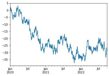
DataFrame에서 plot() method는 모든 column의 data를 간편하게 그래프로 표현할 수 있으며 각 column별로 labeling도 할 수 있습니다.
df = pd.DataFrame(
        np.random.randn(1000, 4),
        index = ts.index,
        columns = ['A', 'B', 'C', 'D']
        )

df = df.cumsum()

plt.figure()
<Figure size 432x288 with 0 Axes><Figure size 432x288 with 0 Axes>
df.plot()<matplotlib.axes._subplots.AxesSubplot at 0x19d00bf8c08>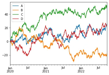
Getting data in/out
생성/분석에 사용하는 data를 파일로 쓰거나 불러오는 방법입니다.
앞서 진행한 import를 반복합니다.
import numpy as np
import pandas as pd
시계열 데이터를 생성한 뒤 csv 파일로 저장해 봅시다.
df = pd.DataFrame(
        np.random.randn(1000, 4),
        index = pd.Series(np.random.randn(1000), index=pd.date_range('1/1/2020', periods=1000)),
        columns = ['A', 'B', 'C', 'D']
        )
df.to_csv('foo.csv')
반대로 csv 파일을 읽어봅시다.
pd.read_csv('foo.csv') Unnamed: 0 A B C D
0 -0.278836 0.207474 0.001968 1.314218 -0.199339
1 0.070793 -0.747281 0.057319 1.140240 1.507255
2 0.620508 -0.361898 -0.663693 0.624234 0.331756
3 0.011931 0.208971 -0.636545 0.346130 -1.738320
4 0.271138 -0.164832 -1.424289 0.257722 -0.438648
.. ... ... ... ... ...
995 -1.457444 -1.197647 -0.930289 0.032803 -0.156479
996 -0.025240 -0.861467 2.008338 0.769440 0.178559
997 0.341979 1.451293 -0.546777 -0.675252 0.392719
998 -1.139901 -0.247459 0.391524 0.321870 0.973132
999 1.208057 -1.950139 -0.638642 0.580319 -0.759484
[1000 rows x 5 columns]HDF5 (Hierarchical Data Format version 5, 대용량 데이터를 저장하기 위한 파일 포맷)로 저장하고 읽을 수도 있습니다.
df.to_hdf('foo.h5', 'df')
pd.read_hdf('foo.h5', 'df') A B C D
-0.278836 0.207474 0.001968 1.314218 -0.199339
0.070793 -0.747281 0.057319 1.140240 1.507255
0.620508 -0.361898 -0.663693 0.624234 0.331756
0.011931 0.208971 -0.636545 0.346130 -1.738320
0.271138 -0.164832 -1.424289 0.257722 -0.438648
... ... ... ... ...
-1.457444 -1.197647 -0.930289 0.032803 -0.156479
-0.025240 -0.861467 2.008338 0.769440 0.178559
0.341979 1.451293 -0.546777 -0.675252 0.392719
-1.139901 -0.247459 0.391524 0.321870 0.973132
1.208057 -1.950139 -0.638642 0.580319 -0.759484
[1000 rows x 4 columns]엑셀 파일로도 저장하고 읽을 수 있습니다.
df.to_excel('foo.xlsx', sheet_name='Sheet1')
pd.read_excel('foo.xlsx', 'Sheet1', index_col=None, na_values=['NA']) Unnamed: 0 A B C D
0 -0.278836 0.207474 0.001968 1.314218 -0.199339
1 0.070793 -0.747281 0.057319 1.140240 1.507255
2 0.620508 -0.361898 -0.663693 0.624234 0.331756
3 0.011931 0.208971 -0.636545 0.346130 -1.738320
4 0.271138 -0.164832 -1.424289 0.257722 -0.438648
.. ... ... ... ... ...
995 -1.457444 -1.197647 -0.930289 0.032803 -0.156479
996 -0.025240 -0.861467 2.008338 0.769440 0.178559
997 0.341979 1.451293 -0.546777 -0.675252 0.392719
998 -1.139901 -0.247459 0.391524 0.321870 0.973132
999 1.208057 -1.950139 -0.638642 0.580319 -0.759484
[1000 rows x 5 columns]